- Home
- Snowflake
- SnowPro Advanced Certification
- DAA-C01
- DAA-C01 - SnowPro Advanced: Data Analyst Exam
Snowflake DAA-C01 SnowPro Advanced: Data Analyst Exam Exam Practice Test
SnowPro Advanced: Data Analyst Exam Questions and Answers
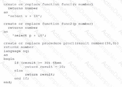
A Data Analyst created two functions and one procedures:
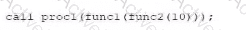
The Analyst then runs this query:
The Analyst then runs this query:
What will be the output?
Options:
Null
10
20
30
Answer:
CExplanation:
To determine the output of the final statement, a Data Analyst must perform a step-by-step trace of the code execution, following standard order of operations (inner-to-outer) and procedural logic within the Snowflake Scripting environment.
Step 1: Evaluating the innermost function, func2(10)
The definition for func2 takes a number p and returns p + 10.
Input: 10
Calculation: $10 + 10 = 20$
Result: 20
Step 2: Evaluating the next function, func1(20)
The definition for func1 takes a number v and returns v + 10.
Input: 20 (the result from Step 1)
Calculation: $20 + 10 = 30$
Result: 30
Step 3: Evaluating the procedure call, proc1(30)
The procedure proc1 takes an input variable named result. It then executes a conditional IF statement:
Conditional Check: IF (result >= 30)
Since the input is 30, the condition evaluates to True.
Action: The procedure executes RETURN result - 10.
Calculation: $30 - 10 = 20$
Summary of Logic:
The nested calls flow as follows: call proc1(30) $\rightarrow$ proc1 evaluates $30 \ge 30$ $\rightarrow$ proc1 returns $30 - 10$, which is 20. If the initial input had been lower, such that the final result passed to the procedure was less than 30, it would have followed the ELSE branch and returned the original value. This question evaluates the analyst's ability to interpret modular code and procedural control flow, which are key components of the Data Transformation and Data Modeling domain in the SnowPro Advanced: Data Analyst exam.
A Data Analyst is working with three tables:
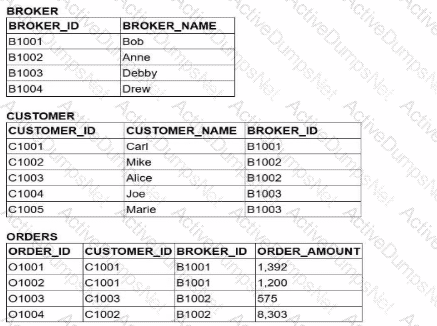
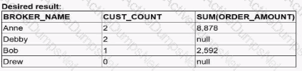
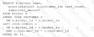
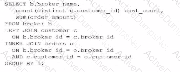
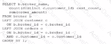
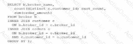
Which query would return a list of all brokers, a count of the customers each broker has. and the total order amount of their customers (as shown below)?
A)
B)
C)
D)
Options:
Option A
Option B
Option C
Option D
Answer:
CExplanation:
To achieve the desired result, an analyst must understand the fundamental behavior of different JOIN types within Snowflake and how they affect the retention of records from the "left" or primary table. The goal here is to list all brokers, even those who have zero customers (like "Drew") or customers with zero orders (like "Debby").
In SQL, an INNER JOIN only returns rows when there is a match in both tables. If we were to use an INNER JOIN between BROKER and CUSTOMER, Drew would be excluded from the results because he has no associated records in the CUSTOMER table. Similarly, an INNER JOIN with the ORDERS table would exclude any broker whose customers haven't placed an order.
Evaluating the Join Logic:
Option C is the correct solution because it utilizes a chain of LEFT JOINs. A LEFT JOIN (or LEFT OUTER JOIN) ensures that every record from the left table (BROKER) is preserved in the result set. If no matching record exists in the joined table (CUSTOMER or ORDERS), Snowflake populates the columns with NULL. This is why "Drew" appears with a CUST_COUNT of 0 and "Debby" appears with a NULL for the total order amount.
Option A fails because it uses an INNER JOIN for the CUSTOMER table, which would immediately filter out "Drew."
Option B and Option D fail because they use INNER JOINs at different stages of the query, which would strip away brokers or customers that do not have matching order activity.
Additionally, the query correctly uses COUNT(DISTINCT c.customer_id) to ensure that customers are not double-counted if they have multiple orders, and GROUP BY 1 (referencing b.broker_name) to aggregate the data at the broker level. This pattern is essential for accurate Data Analysis in Snowflake when dealing with "optional" relationships in a star or snowflake schema.
A Data Analyst created a cost overview dashboard in Snowsight. Management has asked for a system date filter to easily change the time period and refresh the data in all dashboard tiles with a single filter selection.
The system date filter is shown below:
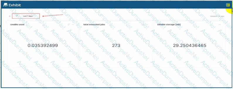
The Analyst wants to apply the filter onto individual dashboard components.
Adding which where clause to the queries will apply the filter as required?
Options:
Where start_time >= dateadd('days', -7, SYSDATE())
Where start_time >= dateadd('days', -7, CURRENT_TIMESTAMP())
Where start_time = :date_filter
Where start_time = :daterange
Answer:
DExplanation:
In Snowsight, the modern web interface for Snowflake, System Filters are specialized keywords that provide out-of-the-box interactivity for dashboards and worksheets. These filters allow non-technical users to manipulate the timeframes of visualizations (e.g., switching from "Last 7 days" to "Last 12 months") without requiring an analyst to manually rewrite the underlying SQL code.
The most critical keyword for temporal filtering is :daterange. When a dashboard contains a date filter widget (as shown in the provided exhibit), the :daterange keyword acts as a dynamic placeholder for the range selected by the user. Unlike a standard variable that might represent a single date, :daterange is specifically designed to handle the start and end boundaries of a period. When injected into a WHERE clause, Snowflake automatically expands this keyword into the appropriate logic to filter records between those two points in time.
Evaluating the Options:
Options A and B are incorrect because they use hard-coded logic (-7 days). While these would return data for the last week, they are static. Changing the filter in the dashboard UI would have no effect on these queries, failing the requirement to "easily change the time period" via the filter selection.
Option C is incorrect because :date_filter is not a reserved system keyword in Snowsight. While an analyst could create a custom filter with that name, it would not automatically link to the standard system date widget shown in the image.
Option D is the 100% correct answer. Using WHERE
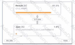
What potential problem can be identified in the Query profile below?
Options:
There is query spilling.
There is an exploding join
There Is inefficient pruning.
The query is not using a foreign Key.
Answer:
BExplanation:
The provided image shows a specific section of a Snowflake Query Profile, which is a visual representation of the execution plan and the actual performance of a query. Analyzing this profile is a critical skill for a Data Analyst to identify performance bottlenecks.
1. Identifying the Exploding Join: The most striking evidence in this profile is the relationship between the input and output row counts of the Join [5] operator.
Input Row Counts: The join receives approximately 95.26k rows from one branch and 150k rows from the other.
Output Row Count: The join produces a staggering 571.6M rows.
When a join operation produces a significantly larger number of rows than the sum of its inputs, it is known as an exploding join (or a "Cartesian product-like" behavior). This typically occurs when the join condition is not restrictive enough or when there are many-to-many relationships with duplicate keys in both joining tables. In this specific case, joining on C1.C_NATIONKEY = C2.C_NATIONKEY has caused the row count to balloon from thousands to over half a billion.
2. Impact on Performance: Exploding joins consume excessive CPU and memory resources to process the massive intermediate result set. This often leads to secondary problems like spilling (Option A), where the data exceeds the virtual warehouse's memory and must be written to disk. However, the profile clearly identifies the join itself as the root cause.
Evaluating the Options:
Option A is a symptom, but the visual evidence of row expansion directly points to the join logic itself.
Option C (inefficient pruning) would be identified by a high percentage of partitions scanned in the Table Scan nodes, not by a row count explosion after a join.
Option D is irrelevant; while foreign keys can help the optimizer, their absence doesn't cause this specific visual profile on its own.
Option B is the 100% correct answer. The "exploded" arrow indicating 571.6M rows leaving a join fed by significantly smaller inputs is the textbook definition of an exploding join.
A Data Analyst needs to generate a graphic that will identify any natural clusters in a data set containing details about completed orders. Which Snowsight chart should be used?
Options:
Line chart
Heat grid
Bar chart
Scatter plot
Answer:
DExplanation:
In the realm of Data Presentation and Data Visualization, selecting the appropriate chart type is critical for revealing the underlying structure of data. When an analyst is tasked with identifying "natural clusters," they are looking for groups of data points that share similar characteristics across two or more dimensions.
A Scatter Plot is the primary visualization tool for this purpose. By plotting two numeric variables (e.g., ORDER_AMOUNT on the X-axis and CUSTOMER_LOYALTY_SCORE on the Y-axis), the scatter plot allows the human eye to immediately detect density. If the data points form distinct "clouds" or groupings, these represent the clusters the analyst is searching for. In Snowsight, scatter plots are highly effective for exploratory data analysis, as they allow analysts to visualize the relationship between variables and spot outliers that may skew statistical summaries.
Evaluating the Options:
Option A is incorrect because Line Charts are designed to show trends over time (sequential data). They connect points in a specific order, which would obscure clustering logic by forcing a temporal connection between unrelated data points.
Option B is incorrect because a Heat Grid (or Heatmap) is best used for comparing categories across two dimensions using color intensity. While it can show high-density areas, it aggregates data into "bins" or cells, which can mask the fine-grained distribution required to see natural, point-based clusters.
Option C is incorrect because Bar Charts are used for comparing discrete categories or showing distributions within a single dimension. They do not effectively show the correlation between two continuous variables needed for cluster identification.
Option D is the 100% correct answer. The Scatter Plot is the standard analytical graphic for cluster detection and correlation analysis within the Snowflake Snowsight interface, providing the necessary granularity to see how individual orders or customers group together in a multi-dimensional space.
A Data Analyst has a very large table with columns that contain country and city names. Which query will provide a very quick estimate of the total number of different values of these two columns?
Options:
SELECT DISTINCT COUNT(country, city) FROM TABLE1;
SELECT HLL(country, city) FROM TABLE1;
SELECT COUNT(DISTINCT country, city) FROM TABLE1;
SELECT COUNT(country, city) FROM TABLE1;
Answer:
BExplanation:
When working with very large tables, calculating the exact number of unique combinations of columns (cardinality) using COUNT(DISTINCT ...) is a resource-intensive operation. It requires the Snowflake query engine to keep an exhaustive list of every unique pair encountered in memory, which can lead to high credit consumption and performance bottlenecks.
To provide a "very quick estimate," Snowflake utilizes the HyperLogLog (HLL) algorithm. The function HLL(column1, column2, ...) returns an HLL state (a binary representation) that can be used to estimate the number of distinct values with a high degree of accuracy and minimal computational overhead. This is part of Snowflake's suite of approximate aggregation functions, which are essential for Data Analysis on massive datasets where a 1% margin of error is acceptable in exchange for significantly faster results.
Evaluating the Options:
Option A is syntactically incorrect; DISTINCT cannot be used in that position with COUNT.
Option C is a valid query but will be significantly slower and more expensive than an HLL estimate on a "very large table".
Option D simply counts the total number of non-null rows, which does not represent the "number of different values" (cardinality).
Option B is the 100% correct answer. It specifically addresses the requirement for a "quick estimate" using the industry-standard probabilistic counting method built into Snowflake.
Which query will provide this data without incurring additional storage costs?
Options:
CREATE TABLE DEV.PUBLIC.TRANS_HIST LIKE PROD.PUBLIC.TRANS_HIST;
CREATE TABLE DEV.PUBLIC.TRANS_HIST AS (SELECT * FROM PROD.PUBLIC.TRANS_HIST);
CREATE TABLE DEV.PUBLIC.TRANS_HIST CLONE PROD.PUBLIC.TRANS_HIST;
CREATE TABLE DEV.PUBLIC.TRANS_HIST AS (SELECT * FROM PROD.PUBLIC.TRANS_HIST WHERE extract(year from (TRANS_DATE)) = 2019);
Answer:
CExplanation:
Snowflake utilizes a unique architecture known as Zero-Copy Cloning, which allows users to create a replica of a table, schema, or entire database without physically duplicating the underlying data files (micro-partitions). When you execute the CLONE command, Snowflake simply creates new metadata that points to the existing micro-partitions of the source object.
Because the data is not physically copied, the clone operation is nearly instantaneous and, crucially, incurs no additional storage costs at the moment of creation. Storage costs only begin to accumulate for the clone when the data in the source or the clone diverges—for example, if rows are updated or deleted in the clone, Snowflake creates new micro-partitions to store the changed data while preserving the original state in the source.
Evaluating the Options:
Option A (LIKE) only copies the column definitions and structure of the table. It does not copy the data itself, so while it doesn't incur storage, it also doesn't provide the "data" requested by the prompt.
Option B (CTAS - Create Table As Select) performs a full deep copy of the data. This creates entirely new micro-partitions, which immediately increases the storage footprint and associated costs.
Option D is a filtered CTAS operation. While it may result in less data than the full table, it still involves creating new physical storage for the 2019 records, thus incurring additional costs.
Option C is the 100% correct answer. It uses the CLONE keyword, which is the specific Snowflake feature designed to provide a full dataset for dev/test environments with zero initial storage impact. This is a core competency in the Data Transformation and Data Modeling domain.
A large, complicated query is used to generate a data set for a report on the most recent month. It is taking longer than expected. A review of the Query Profile shows excessive spilling. How can the performance of the query be improved WITHOUT increasing costs?
Options:
Run the query against zero-copy clones of the source tables to avoid contention with other queries.
Create a materialized view clustered on a date column, on the table that is causing the spilling.
Change the source tables into external tables to establish and take advantage of custom partitioning.
Split the query into multiple steps, replacing Common Table Expressions (CTEs) with temporary tables to process the data in smaller batches.
Answer:
DExplanation:
In Snowflake, "spilling" occurs when the intermediate data required to process a query exceeds the available memory (RAM) of the virtual warehouse. When this happens, Snowflake "spills" the data first to the warehouse's local SSD and, if that fills up, to remote storage (e.g., S3 or Azure Blob). This significantly degrades performance due to increased I/O latency.
To resolve this without increasing costs (i.e., without scaling up to a larger warehouse size), an analyst must reduce the memory footprint of the query.
CTEs vs. Temporary Tables: While Common Table Expressions (CTEs) are excellent for readability, they are often treated as logical entities that the optimizer may re-evaluate multiple times or struggle to keep in memory during massive joins.
Batch Processing: By splitting a single monolithic query into multiple steps and storing intermediate results in temporary tables, the analyst forces the engine to clear its memory between steps. This process acts as a "checkpoint," effectively processing the data in smaller, more manageable batches that fit within the current warehouse's memory limits.
Evaluating the Options:
Option A is incorrect because spilling is a compute-resource issue, not a storage-lock or contention issue.
Option B is incorrect because materialized views and clustering incur background credit costs for maintenance, violating the "without increasing costs" constraint.
Option C is incorrect because external tables are generally slower than native Snowflake tables due to the lack of proprietary metadata and micro-partitioning.
When building a Snowsight dashboard that will allow users to filter data within a worksheet, which Snowflake system filters should be used?
Options:
Include the :datebucket system filter in a WHERE clause, and include the :daterange system filter in a GROUP BY clause.
Include the :daterange system filter in a SELECT clause, and include the :datebucket system filter in a GROUP BY clause.
Include the :datebucket system filter in a WHERE clause, and include the :daterange system filter in a SELECT clause.
Include the :daterange system filter in a WHERE clause, and include the :datebucket system filter in a GROUP BY clause.
Answer:
DExplanation:
Snowsight provides special System Keywords that allow analysts to create dynamic, interactive dashboards without hard-coding dates. Two of the most critical keywords are :daterange and :datebucket.
The :daterange keyword is designed to filter the volume of data based on a time period selected by the user in the dashboard UI (e.g., "Last 30 days" or "Current Year"). Because it acts as a filter on the underlying data, it must be placed in the WHERE clause of the SQL statement (e.g., WHERE created_at = :daterange). This ensures that only the records within the selected timeframe are processed by the query.
The :datebucket keyword is used for time-series aggregation. It allows the user to dynamically change the granularity of the data—for example, switching a chart from "Daily" to "Monthly" views without rewriting the query. To achieve this, :datebucket is used inside a date-truncation function in the SELECT list and, crucially, must be included in the GROUP BY clause to correctly aggregate the metrics (e.g., GROUP BY 1 or GROUP BY :datebucket).
Evaluating the Options:
Option A is incorrect because :datebucket is for grouping/truncation, not for filtering in a WHERE clause.
Option B is incorrect because :daterange is a filter (returning a range), not a scalar value suitable for a SELECT list.
Option C is incorrect for the same reasons as A and B.
Option D is the 100% correct answer. It follows the standard Snowsight design pattern: :daterange restricts the data rows in the WHERE clause, while :datebucket defines the temporal aggregation level in the GROUP BY clause.
Table TB_A with column COL_B contains an ARRAY. Which statement will select the last element of the ARRAY?
Options:
SELECT GET(COL_B, ARRAY_SIZE(COL_B)-1) FROM TB_A;
SELECT COL_B[ARRAY_SIZE(COL_B)] FROM TB_A;
SELECT COL_B[-1] FROM TB_A;
SELECT LAST_VALUE(COL_B) FROM TB_A;
Answer:
AExplanation:
Working with semi-structured data types like Arrays is a core competency for a Snowflake Data Analyst. In Snowflake, arrays are zero-indexed, meaning the first element is at position 0. Consequently, the index of the last element is always the total number of elements minus one ($Size - 1$).
To retrieve an element from a specific index, Snowflake provides the GET() function. This function takes the array column and the calculated index as arguments. When combined with ARRAY_SIZE(), which returns the total count of elements in the array, the formula ARRAY_SIZE(COL_B)-1 accurately targets the final index regardless of the array's length.
Evaluating the Options:
Option B is incorrect because using ARRAY_SIZE as the index directly (without subtracting 1) results in an "out-of-bounds" error or returns NULL, because the index equals the length (e.g., in an array of 3 items, the max index is 2).
Option C is incorrect. While some programming languages (like Python) allow negative indexing to start from the end, Snowflake SQL does not support this shorthand for arrays; it would simply return NULL.
Option D is incorrect because LAST_VALUE is an Analytic/Window function used to find the last row in a sorted result set, not the last element within a single array cell.
Option A is the 100% correct approach. It uses the standard, robust method for dynamic index calculation. This ensures that even if different rows have arrays of different lengths, the query will always successfully "pluck" the final item from each. This skill is vital for Data Transformation tasks, such as extracting the most recent status from a history array.
A Data Analyst creates and populates the following table:
create or replace table aggr(v int) as select * from values (1), (2), (3), (4);
The Analyst then executes this query:
select percentile_disc(0.60) within group (order by v desc) from aggr;
What will be the result?
Options:
1
2
3
4
Answer:
BExplanation:
The PERCENTILE_DISC (discrete percentile) function is an inverse distribution function that assumes a discrete distribution model. It takes a percentile value and a sort specification and returns the value from the set that corresponds to that percentile. Unlike PERCENTILE_CONT, which interpolates between values to find a continuous result, PERCENTILE_DISC always returns an actual value from the input set.
In this scenario, we have a set of four values: $\{1, 2, 3, 4\}$. The query specifies a descending order (order by v desc), so the ordered set for the calculation is $\{4, 3, 2, 1\}$.
To find the discrete percentile, Snowflake calculates the cumulative distribution. For a set of $N$ elements, each element represents a percentile rank of $1/N$. With 4 elements, each covers 25% ($0.25$) of the distribution:
Value 4: Cumulative Percentile $0.25$
Value 3: Cumulative Percentile $0.50$
Value 2: Cumulative Percentile $0.75$
Value 1: Cumulative Percentile $1.00$
The PERCENTILE_DISC(0.60) function looks for the first value whose cumulative distribution is greater than or equal to the specified percentile ($0.60$).
$0.25$ (Value 4) is not $\ge 0.60$.
$0.50$ (Value 3) is not $\ge 0.60$.
$0.75$ (Value 2) is the first value where the cumulative distribution is $\ge 0.60$.
Therefore, the result is 2. If the order had been ascending (ASC), the cumulative distribution would have been $\{1: 0.25, 2: 0.50, 3: 0.75, 4: 1.00\}$, and the result for $0.60$ would have been 3. Understanding the impact of the ORDER BY clause within the WITHIN GROUP syntax is a critical skill for the Data Analysis domain of the SnowPro Advanced: Data Analyst exam.
A Data Analyst runs a query in a Snowflake worksheet, and selects a numeric column from the result grid. What automatically-generated contextual statistic can be visualized?
Options:
A histogram, displayed for all numeric, date, and time columns
A frequency distribution, displayed for all numeric columns
MIN/MAX values for the column
A key distribution
Answer:
AExplanation:
One of the standout features of the Snowsight interface is its ability to perform automatic Data Profiling. When a Data Analyst executes a query, Snowflake doesn't just return a raw grid of data; it analyzes the result set to provide immediate visual insights.
When you click on a column header in the results pane, a summary statistics panel appears. For numeric, date, and time columns, Snowflake automatically generates a histogram (Option A). This histogram provides a visual representation of the data distribution, allowing the analyst to quickly identify patterns, concentrations of values, or significant outliers without writing additional SQL code.
Evaluating the Options:
Option B: While a histogram is a type of frequency distribution, Option A is more accurate because Snowsight also provides these visualizations for date and time types, not just integers/floats.
Option C: While MIN and MAX values are displayed in the summary panel, they are text-based statistics, not the "visualized" contextual statistic (the histogram) emphasized in the question.
Option D: "Key distribution" is not a standard visualization term used in the Snowsight profiling tool.
Option A: Is the 100% correct answer. It highlights the breadth of the profiling tool (covering numbers, dates, and times) and the specific visual element (the histogram) that makes exploratory data analysis significantly faster for a Data Analyst.
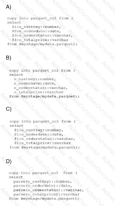
A Data Analyst has a Parquet file stored in an Amazon S3 staging area. Which query will copy the data from the staged Parquet file into separate columns in the target table?
Options:
Option A
Option B
Option C
Option D
Answer:
CExplanation:
In the Snowflake ecosystem, Parquet is treated as a semi-structured data format. When you stage a Parquet file, Snowflake does not automatically parse it into multiple columns like it might with a flat CSV file. Instead, the entire content of a single row or record is loaded into a single VARIANT column, which is referenced in SQL using the positional notation $1.
The fundamental mistake often made—and represented in Option A—is treating Parquet as a delimited format where $1, $2, and $3 refer to different columns. In Parquet ingestion, columns $2 and beyond will return NULL because the schema is contained within the object in $1.
To successfully "shred" or flatten this semi-structured data into a relational table with separate columns, an analyst must use path notation. This involves referencing the root object ($1), followed by a colon (:), and then the specific element key (e.g., $1:o_custkey). Furthermore, because the values extracted from a Variant are technically still Variants, they must be explicitly cast to the correct data type using the double-colon syntax (e.g., ::number, ::date) to ensure they land in the target table with the correct data types.
Evaluating the Options:
Option A is incorrect because it uses positional references ($2, $3, etc.) which are only valid for structured files like CSVs.
Option B is incorrect because it attempts to reference keys directly without the required stage variable ($1) and colon separator.
Option D is incorrect as it uses a non-standard parse() function that does not exist for this purpose in Snowflake SQL.
Option C is the 100% correct syntax. It correctly identifies that the Parquet data resides in $1, utilizes the colon to access internal keys, and applies the necessary type casting. This specific method is known as "Transformation During Ingestion" and is a core competency for any SnowPro Advanced Data Analyst.
A Data Analyst is creating a Snowsight dashboard from a shared worksheet. What happens to the access and permissions of the users who initially had sharing privileges on the worksheet?
Options:
The original users retain access and permissions on the worksheet.
The original users gain additional access to the worksheet.
The original users temporarily lose access but regain it once the dashboard is created.
The original users lose access to the worksheet, their permissions on the worksheet are revoked.
Answer:
DExplanation:
When working within the Snowsight interface, the transition from a standalone worksheet to a dashboard component involves a change in how the underlying SQL and its associated metadata are managed. When a worksheet is converted or used to create a dashboard, the ownership and sharing model shifts to the dashboard level.
According to Snowflake's documentation on Snowsight collaboration, when a user creates a dashboard from a worksheet that was previously shared with others, the original worksheet's individual share settings are essentially superseded by the dashboard's own permissions. In many workflow scenarios within the UI, once the worksheet is finalized into a dashboard tile, the direct, independent access to that specific worksheet is severed for the original "sharees." Their permissions on that specific worksheet are revoked to prevent conflicting edits between the standalone version and the dashboard-integrated version.
Evaluating the Options:
Option A is incorrect because Snowsight manages the lifecycle of worksheets used in dashboards as part of the dashboard object; independent sharing of the underlying worksheet is typically disabled or revoked.
Option B and C are distractors; there is no mechanism in Snowsight that grants "additional" access or "temporary" loss during the creation process.
Option D is the 100% correct answer based on the SnowPro Data Analyst standard regarding Snowsight object ownership and sharing lifecycle. To allow others to see the work, the Analyst must now share the Dashboard itself, rather than relying on the previous worksheet-level permissions. This ensures a "single source of truth" for the visualization's logic.
A Data Analyst executes a complex query. Which query will allow the Analyst to access the results a second time?
Options:
SELECT * FROM TABLE(RESULT_SCAN(LAST_QUERY_ID()));
SELECT * FROM TABLE(INFORMATION_SCHEMA.QUERY_HISTORY());
DESC RESULT LAST_QUERY_ID();
SELECT LAST_QUERY_ID(-1);
Answer:
AExplanation:
Snowflake provides a powerful feature called Result Caching. When a query is executed, the results are persisted for 24 hours. To access the result set of a previously executed query without re-running the heavy computation (and thus saving credits), a Data Analyst can use the RESULT_SCAN table function.
The function RESULT_SCAN requires a Query ID as its input. The most common way to programmatically retrieve the ID of the most recently executed statement in the current session is by using the LAST_QUERY_ID() function. By wrapping this in the TABLE() operator, Snowflake treats the cached results as a virtual table that can be queried, filtered, or even joined with other tables.
Evaluating the Options:
Option B is incorrect because QUERY_HISTORY returns metadata about queries (like start time, user, and status) but does not return the actual data records produced by those queries.
Option C is incorrect as DESC (Describe) is used to see the columns and data types of an object, not to fetch its row data.
Option D is incorrect; while LAST_QUERY_ID(-1) might successfully retrieve a string representing a previous ID in some contexts, it does not actually "access the results" or display the data.
Option A is the 100% correct syntax. It is the standard method used by Data Analysts to perform post-processing on a large result set or to recover a result set if the worksheet was accidentally cleared. This is a key part of the Data Analysis domain, specifically regarding performance optimization and the utilization of Snowflake's unique caching layers.
What option would allow a Data Analyst to efficiently estimate cardinality on a data set that contains trillions of rows?
Options:
Count(Distinct *)
HLL(*)
SYSTEM$ESTIMATE
Count(Distinct *)/Count(*)
Answer:
BExplanation:
When working with "Big Data" at the scale of trillions of rows, calculating an exact count of unique values using COUNT(DISTINCT column) is extremely resource-intensive. This is because Snowflake must keep track of every unique value encountered to ensure no duplicates are counted, leading to high memory usage and long execution times (often referred to as "spilling to disk").
To solve this, Snowflake provides HyperLogLog (HLL) functions. HLL(*) (or specifically HLL_ACCUMULATE and HLL_ESTIMATE) allows an analyst to estimate the cardinality (the number of unique elements) with a very small, known margin of error (typically around 1%). This is significantly faster and uses far fewer credits than an exact count because it uses a probabilistic algorithm rather than a state-heavy tracking mechanism.
Evaluating the Options:
Option A is technically correct for small datasets but is highly inefficient for trillions of rows, directly contradicting the "efficiently" requirement of the question.
Option C is a distractor; while Snowflake has various SYSTEM$ functions, SYSTEM$ESTIMATE is not a standard function for cardinality.
Option D is a formula that doesn't target cardinality but rather a ratio (density).
Option B is the correct answer. The HLL family of functions is the industry standard within Snowflake for high-performance cardinality estimation on massive datasets.
A Data Analyst needs to temporarily hide a tile in a dashboard. The data will need to be available in the future, and additional data may be added. Which tile should be used?
Options:
Show/Hide
Duplicate
Delete
Unplace
Answer:
DExplanation:
In Snowsight, managing dashboard layouts requires an understanding of how tiles (queries or visualizations) are stored versus how they are displayed. When an analyst wants to remove a tile from the visible dashboard grid without destroying the underlying query logic or historical configuration, the Unplace action is the correct functional choice.
When a tile is unplaced, it is removed from the dashboard's active layout but remains part of the dashboard's "library" of available content. This is a critical distinction from the Delete action (Option C), which permanently removes the tile and its associated SQL code from the dashboard object. Unplacing allows the analyst to "archive" the work temporarily. Because the tile still technically exists within the dashboard's metadata, any new data added to the underlying tables will still be processed by the query whenever the tile is eventually placed back onto the grid.
Evaluating the Options:
Option A (Show/Hide) is not a standard standalone command for dashboard tile management in Snowsight; visibility is typically managed through placement on the grid.
Option B (Duplicate) creates a second copy of the tile. While this preserves the data, it does not satisfy the requirement to "hide" the current tile; it actually adds more clutter to the dashboard.
Option C (Delete) is incorrect because the prompt specifies that the data and tile will need to be available in the future. Deleting would require the analyst to rewrite the SQL and reconfigure the visualization from scratch.
Option D is the 100% correct answer. Unplacing is the "soft-remove" feature of Snowsight. It preserves the tile in the "Unplaced Tiles" sidebar, allowing for quick restoration at a later date. This feature is essential for analysts who need to manage evolving reporting requirements where certain metrics may only be relevant seasonally or during specific business cycles.
Which Snowflake SQL would a Data Analyst use in a trained Cortex model named forecast_model to retrieve the components that contribute to the predictions?
Options:
forecast_model!SHOW_EVALUATION_METRICS()
forecast_model!SHOW_TRAINING_LOGS()
forecast_model!EXPLAIN_FEATURE_IMPORTANCE()
forecast_model!FORECAST()
Answer:
CExplanation:
Snowflake Cortex ML functions, such as the Forecasting and Anomaly Detection models, are designed to be "black boxes" that provide automated machine learning capabilities directly within SQL. However, for a Data Analyst to trust and validate these models, Snowflake provides specific Object Methods (invoked with the ! operator) to inspect the model's internal logic and performance.
The !EXPLAIN_FEATURE_IMPORTANCE() method is specifically designed to provide transparency into how the model reached its conclusions. When invoked on a trained forecast model, it returns a result set showing which features (such as exogenous variables or time-based components like seasonality and trend) had the most significant impact on the predicted values. This is a critical step in the Data Analysis workflow to ensure that the model is not relying on "noise" or irrelevant data points.
Evaluating the Options:
Option A (SHOW_EVALUATION_METRICS) is used to retrieve accuracy statistics like MSE (Mean Squared Error) or MAPE (Mean Absolute Percentage Error) from the training phase, but it does not explain the contribution of specific features.
Option B (SHOW_TRAINING_LOGS) is not a standard Cortex ML method; logging details are typically handled internally or through different system views.
Option D (FORECAST) is the primary method used to actually generate the future predictions once the model is trained; it outputs the forecast itself, not the underlying component importance.
Option C is the correct answer as it is the dedicated method for model interpretability, allowing analysts to see the "why" behind the forecast by quantifying the influence of each input variable. This aligns with Snowflake's focus on "Explainable AI" within the Data Cloud.
This command was executed:
SQL
SELECT seq4(), uniform(1, 10, RANDOM(12))
FROM TABLE(GENERATOR(TIMELIMIT => NULL))
ORDER BY 1;
How many rows will be generated?
Options:
An infinite number
12
10
0
Answer:
DExplanation:
The GENERATOR table function is used in Snowflake to produce a synthetic result set, typically for testing or creating dummy data. However, the GENERATOR function requires at least one of two parameters to be explicitly set to a positive value to produce any rows: ROWCOUNT or TIMELIMIT.
In the provided query, the user has set TIMELIMIT => NULL. In Snowflake's SQL implementation for the GENERATOR function, NULL is treated as a zero or an undefined limit. Furthermore, since the ROWCOUNT parameter is omitted, it defaults to zero. Because neither a positive duration nor a positive row count has been specified, the generator engine has no instruction on how many rows to build.
Evaluating the Results:
Option A is a distractor; while one might think NULL means "no limit" (infinity), the GENERATOR function is designed to be finite and safe.
Option B is incorrect; the number 12 inside the RANDOM(12) function is merely a seed value for the random number generator, ensuring the output is reproducible. It has no impact on the number of rows produced by the FROM clause.
Option C is incorrect; 10 is just a boundary for the UNIFORM function.
Option D is the 100% correct answer. Because the query specifies TIMELIMIT => NULL and fails to provide a ROWCOUNT, Snowflake will execute the query successfully but return a result set containing 0 rows. This is a common "trick" question in the Data Analysis domain to test an analyst's familiarity with table function parameters.
Unlock DAA-C01 Features
- DAA-C01 All Real Exam Questions
- DAA-C01 Exam easy to use and print PDF format
- Download Free DAA-C01 Demo (Try before Buy)
- Free Frequent Updates
- 100% Passing Guarantee by Activedumpsnet
Questions & Answers PDF Demo
- DAA-C01 All Real Exam Questions
- DAA-C01 Exam easy to use and print PDF format
- Download Free DAA-C01 Demo (Try before Buy)
- Free Frequent Updates
- 100% Passing Guarantee by Activedumpsnet